

As known, synthetic geometry is a foundation of explorations in analytic geometry. It is proved by sayings of G. Kantor [1]: «…for a long time complications arose at the way of introducing complex values, before their geometric presentation with points and ranges on a plane has been found»; and F. Klein [2]: «…historical emergence of the idea of irrational values has its roots in geometric intuition», etc.
In his work, F. Klein specifies: «...two types of geometry are outlined: synthetic geometry…and…analytic geometry… A third type can be studied besides these two, ..it is a generalization of the first two types». It is known that one of synthetic geometries is called descriptive geometry that studies methods of displaying spatial forms onto a plane.
The display process includes:
– an original;
– display apparatus;
– a model (an image);
– model bearer.
Any spatial objects serve as an original, a point is the simplest one of them, it is explicitly defined by three coordinates with regularity ∞3 (a point on a plane has regularity ∞2, a point on a curve (straight) has regularity ∞1) [4].
Curved (straight) lines or surfaces (planes) can serve as projecting apparatus.
A model (image) of a point will be represented by a point while projecting with a curved (straight) line or a curve (straight) while projecting with a surface (plane).
A surface (plane) or a curved (straight) line can serve as a bearer of the model.
To express the provided information, we will take a point as an original, in other words:
A point is the original
An original is a point
cluster (S) or clusters of straights are the display apparatus
a point or points are the model
a plane is the model bearer.
Besides, a necessary requirement while projecting a space point that has regularity is that its model has the same regularity ∞3.
Clusters of straights (S1) and (S2)are the projecting apparatus, and plane P is the model bearer. Space point A is projected form the center of S1 to the point A1 on the plane P (Fig. 1) that has regularity ∞2, and all points of the beam SA1 are projected into the point A1. In order to meet the projection requirement, we take another projection center S2, and points S1 and S2 will define the straight in the space, and it will cross the plane P in point F0 that is constant for this projections apparatus and will discharge beam of straights (F0) on the plane P. Then, A1 will discharge the straight from the beam of straights (F0), and onto it we will project the point A from the center S2 into the point A2 with regularity ∞1. As a result, we will have a model of point A on the plane P – a couple of points A1 and A2, in other words, the model regularity will equal  and here we can see that regularities of the original and the received model are equal.
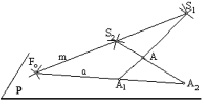
Fig. 1
If a body will serve as an original, it will separate into cut-offs as a beam (m). The cut-offs will model from projection centers (S1) and (S2) in the beam of straights (F0) on the plane P.
Thus, descriptive geometry solves two problems: a direct problem – receiving a model of an original via projection apparatus according to the given original; and an indirect problem – receiving an original via projection apparatus according to a given model. The direct problem of descriptive geometry is called modeling, and the indirect problem is called constructing.
Let us explain the process of modeling and constructing, using Fig. 1.
We model point A via projection apparatus with two beams of straights аппаратом (S1) and (S2) onto the surface P. Projection centers S1 and S2 will define the line m in space, and it will cross the plane P in point F0 that defines the beam of straights (F0) on the plane P. Modeling space point A is carried out in the plane Δ(A, m). Point A from the center S1 is projected into the point A1 that defines, for example, the straight a from the beam of straights (F0). On it we will project the point A from the center S2 into the point A2. As a result, model of the point A is represented by the couple of points A1 and A2.
Construction of the space point A is carried out if the point model that is a couple of points A1 and A2 on the plane P and projection apparatus, for example, couple of beams of straights (S1) and (S2) in space, is given. As earlier, projection centers S1 and S2 will define the straight m in space, and it will cross the plane P in the point F0 that defines the beam of straight bearers of space points (F0). The given points A1 and A1 lie on one of the straights of the beam of straights (F0), they can lie on the straight a, for example. Crossing straights a and m define the plane Σ(a, m) – the plane of constructing the point A. Beams of projecting the point A1 from the projection center S1 and the point A2 from the center S1 that lie in the plane Σ(a, m)will cross in one point A. Therefore, we can see that the original can be constructed having two model projections.
On the plane P projections of space points will come in to types that we will explain in Fig. 2, 2’.
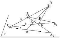
Fig. 2
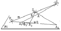
Fig. 2’
We model two points A and B from centers S1 and S2on the plane P. Points A and B will discharge two planes from the beam of planes (m), and these planes will cross the plane P along straights a and b of the beam of straights (F0) (Fig. 2). From the projection center points A and B are projected correspondingly by the pair of points A1 and A2 on the straight на a and B1 and B2 on the straight b. A specific case of placing spatial points A and B is possible. These points can be located on one beam of straight cluster (S1) or (S2). In this case points A and B will belong to one plane of the beam of planes (m), and this plane will be by two crossing straights m and (AB)(). This plane will cross place P along the straight a = b of the beam of straights (F0) (Fig. 2). Points A and B from the projection center S1 will project into the concurred projections A1 = (B1), such point on a projection plane are called rival [5, 6]. Projections of points A and B from the projection center S2 project onto the plane P into two different points A2 and B2 of the straight line a = b.
Emergence of a problem
Let us study implementation of descriptive geometry methods in order to solve some problems of analytic geometry. To do it, let us examine affine coordinates on a plane.
The simplest coordinate system on a straight can be imagined, if we set a starting point on it, point O, a unit with coordinate 1, and positive or negative spacings x from point O (Fig. 3).
On the plane or in space we will take two or three coordinate straights x, y or x, y, z with a mutual point О and random angles that are formed between these straights. Angles that are formed between axis equal 90°. Affine straight is unlimited in both directions, but we will never achieve any point that lies on the opposite direction on it.
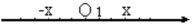
Fig. 3
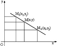
Fig. 4
The special feature of an affine plane is that parallel straights do not cross on it.
On the affine straight let us study the division of the section M1M2 by the straight point M in this relation of m/n, where and are random numbers (Fig. 4). Coordinates of the point M(x, y)according to the coordinates of points M(x1, y1) and M(x2, y3)are produced in textbooks on analytic geometry [7, 8, 9], where 
 for the point M that lies inside the section and (m/n) > 0, if point M will lie outside of the section, (m/n) < 0. If m/n = 1, point M with coordinates
  and
and  will divide the section M1M2 in halves. If m/n = –1, coordinates of the point M′ will be x = ∞ and y = ∞, such points are called unlimitedly remote, and are not studied in affine geometry. These unlimitedly remote points have been introduced into geometry as nonintrinsic elements.
Thus, a nonintrinsic point is produced on a straight, and nonintrinsic is produced on a plane, and nonintrinsic is produced in space. Therefore, each straight obtains a nonintrinsic point that is represented on a closed line (Fig. 5). Now parallel straights have obtained a mutual nonintrinsic point. Producing nonintrinsic points on a straight allowed us to simplify many suggestions, for example, two straights cross on a plane now. Therefore, it is claimed that, while moving in any direction, along a straight we can return to an initial point through the unlimited one. Such straight has been called projective straight, and plane – projective plane, and space – projective space. Studying the problem of dividing the section of the straight M1M2 in relation to m/n on the projective straight, point M∞(∞) in now legalized, and we can suggest that it divides the section M1M∞M2 in relation m/n = –1.
Besides, nonintrinsic geometric images cannot be set with affine coordinates. Therefore, a new definition of coordinates is introduced. It is set for the straight so that each point on the straight has not one, but two corresponding coordinates x1 and x2, we have a redundancy of coordinates for a straight [3]. Moreover, a multiplicity of value systems will be set in correspondence to a single point on a straight, they will be represented as (ρx, ρy), for example, point x – 1. I in the Fig. 6 where ρ is random but not equal to zero number, x1, x2 obtain any values except for their simultaneous equality to zero. In this case we receive a specific single point on a straight, and in case x2 = 0 and x1 = λ we receive a nonintrinsic or unlimited point. Thus produces coordinates are called homogeneous coordinates.
Rival points
Let us study the coordinate  on axis Ox more carefully, where x1 and x2 alter from 0 to ∞ and, it is necessary to consider that while x1 grows and x2 remains constant, x grows, and if x1 remains constant, and x2 grows, x decreases. Let us place variables x, x1, x2 on straights, x – on a horizontal straight, and variables x1 and x2 on parallel straights with an inverse count from the center of axis.
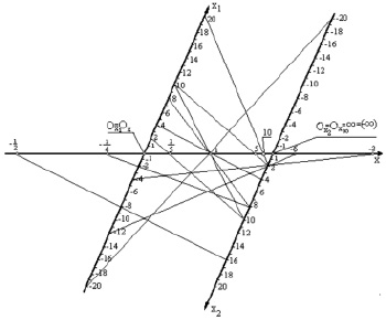
Fig. 5
Let us place the point on infinity within the limits of our sight, it will be the point of crossing between axis Ox2 and Ox, then we will examine the behavior x in this case.
Therefore, we can add a theorem to the claim by G. Kantor on that the point ∞ is the only one on a projective straight [3]: Two point of space ∞ and –∞ project into rival point on a projective straight.
Let us study alterations of on the axis (Fig. 5), it decreases from ∞ to 0, and further to –∞. Therefore, the highest valuedecreases down to the smallest value ∞ on a digital axis. However, –∞ cannot transfer toand backwards. In the Fig. 6 we can see that ∞ closes with the point  on the right, and point –∞ – on its left, and these points coincide with the point
  . In other words, projection of points ∞ and –∞on a projective straight are rival points (it can be observed in Fig. 2’ with points A1 = (B1). Therefore, an original of the projective straight will be represented as a broken spatial curve.
If now values of x increase from x = 0 to ∞ in point  , values of will decrease to the left of zero in point
  down to –∞ in point
  .
.
In case straights (2, –2), (–3, 3), (10, –10) etc. are parallel to the axis and are straight of beam of straights M∞(–1) point x = –1 will be located in the infinity.
Thus, it is obvious that there is no point  on axis Ox.
According to the provided information, we can see that, in order to construct pint on a projective straight, one has to escape to a plane. Two planes are required to construct points on a plane where two axis – Ох and Оу operate, in other words,  and
and  require two planes, and their crossing line will care Ox3 and axis Ох and Оу will be parallel to it.
Since the studied projective straight is a model of a spatial object, we cannot construct it, as a projective straight has only one projection. Each point of an original of a projective straight projects into one point on the model, and only two points –∞ and –∞ project into rival points. There are several spatial lines, and one projection of them represents a closed line with two rival points, for example, a wind of a helical cylindrical line, if ∞ and –∞have been placed at the end and the beginning of the wind while projecting it by a beam of straights with their center in a nonintrinsic point (Fig. 6), or a wind of cone helical line that is projected by a beam of straights from point S that coincides with the cone vertex (Fig. 7). A wind of a helical line that is placed on an unilocular hyperboloid will have a similar projection.
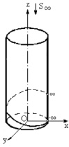
Fig. 6
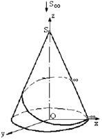
Fig. 7
Resume
Thus, we have geometrically proved that:
1) projections of spatial points ∞ and –∞are rival point on a projective line;
2) x1 and x2cannot equal zero simultaneously, as there is no such point on axis Ox;
3) There is no point  on an affine straight in homogeneous if x1 = –x2 or –x1 = x2.This point exists on a projective straight in point M∞(–1).
Therefore, using methods of descriptive geometry, one can describe an original of a projective straight:
a) An original of a projective straight can be located on: a cone surface with its vertex in point S1 and a directing projective straight, if a projective apparatus will consist of two beams of straights with intrinsic centers S1 and S2. Each point of an original will lie on one forming line of a conic surface, points ∞ and –∞ will lie on the same forming line of a conic surface.
b) An original of a projective straight can lie on a cylindrical surface with a directing projective straight and projection apparatus that consists of two beams of straights with centers  and
and  in nonintrinsic points.
The work was submitted to the International Scientific Conference «Production technologies», Italy (Rome – Florence), September, 7–14, 2013, came to the editorial office оn 14.08.2013.
Библиографическая ссылка
Vertinskaya N.D. On some geometric aspect of interpreting homogeneous coordinates // Международный журнал экспериментального образования. – 2013. – № 12. – С. 78-82;URL: https://expeducation.ru/ru/article/view?id=4300 (дата обращения: 24.04.2024).